Chapter 8 Power Analysis
In this section we provide examples of how we assess statistical power for different experimental research designs. We often prefer to use simulation to assess the power of different research designs because we rarely have designs that fit easily into the assumptions made by analytic tools.
However, for the sake of an example, we will show a version that uses simulation that produces the same answer as the faster analytic version.
Imagine that we thought that a study would have an effect of about 1 standard deviation – this is more or less the effect difference we have created in our example dataset so far. How large a study do we need in order to distinguish this effect from noise?
population <- declare_population(dat1)
potentials <- declare_potential_outcomes(Y ~ Z * y1 + (1 - Z) * y0)

assignment <- declare_assignment(Z = complete_ra(N))
reveal <- declare_reveal(Y, Z)
design <- population + potentials + assignment + reveal

simdat1 <- draw_data(design)

# Notice that we have new potential outcomes called Y_Z_1 and Y_Z_0 that are
# copies of y0 and y1
stopifnot(with(simdat1, cor(y0, Y_Z_0)) == 1)

estimand <- declare_inquiry(ATE = mean(Y_Z_1 - Y_Z_0))
estimator <- declare_estimator(Y ~ Z, inquiry = estimand, label = "Simple D-I-M")

# We can see how the estimator function works using some data simulated based on
# the design
estimator(simdat1)
estimator term estimate std.error statistic p.value conf.low conf.high df outcome inquiry
1 Simple D-I-M Z 5.571 0.8153 6.834 7.069e-10 3.953 7.189 98 Y ATEdesignPlusEst <- design + estimand + estimatorNow that the setup is complete, we can assess the statistical power of our proposed design with \(N=100\) and an effect of roughly 1 SD. The output below shows the statistical power as well as the false positive rate (called “Coverage” below) as well as the difference between the mean difference we calculate and the true average treatment effect (called “Bias” below).
diagnose_design(designPlusEst, sims = 1000)
Research design diagnosis based on 1000 simulations. Diagnosis completed in 5 secs. Diagnosand estimates with bootstrapped standard errors in parentheses (100 replicates).

        Design Inquiry    Estimator Term N Sims Mean Estimand Mean Estimate   Bias SD Estimate
 designPlusEst     ATE Simple D-I-M    Z   1000          5.45          5.47   0.02        0.71
                                                       (0.00)        (0.02) (0.02)      (0.02)
   RMSE  Power Coverage
   0.71   1.00     0.97
 (0.02) (0.00)   (0.01)
The analytic approach suggests more power than the simulation based approach – a difference that we suspect arises from our fairly skewed outcome.
power.t.test(n = 100, delta = 1, sd = 1)
     Two-sample t test power calculation

              n = 100
          delta = 1
             sd = 1
      sig.level = 0.05
          power = 1
    alternative = two.sided

NOTE: n is number in *each* group
For ways to compare different sample sizes, effect sizes, etc. see more information from the DeclareDesign package.
8.1 An example of the off-the-shelf approach
To demonstrate how a power analysis might work in principle, consider another
example using the R function power.t.test().
When using this function, there are three parameters that we’re most concerned with, two of which are specified by the user, and the third of which is then calculated and returned by the function. These are:
n= sample size, or number of observations;,delta= the target effect size, or a minimum detectable effect (MDE); andpower= the probability of detecting an effect if in fact there is a true effect of sizedelta.
Say, for example, you want to know the MDE for a two-arm study with 1,000
participants. Using power.t.test() you would specify:
power.t.test(
  n = 500, # n denotes the number of obs. per treatment arm
  power = 0.8 # use traditional power threshold of 80%
)
     Two-sample t test power calculation

              n = 500
          delta = 0.1774
             sd = 1
      sig.level = 0.05
          power = 0.8
    alternative = two.sided

NOTE: n is number in *each* group
If we wanted to extract the MDE we could write:
power.t.test(
  n = 500, # number of obs. per treatment arm
  power = 0.8 # traditional power threshold of 80%
)$delta
[1] 0.1774We can similarly extract other parameters, like sample size and power, using
$n or $power instead of $delta. If you need to, you can adjust other
parameters, like the standard deviation of the response, the level of the test,
or whether the test is one-sided rather than two-sided. There are also other
functions available for different types of outcomes. For example, if you have a
binary response, you can use power.prop.test() to calculate power for a
difference in proportions test.
An equivalent approach in Stata is as follows:
power twomeans 0, power(0.8) n(1000) sd(1)Stata users can learn more about available tools by checking out Stata’s plethora of relevant help files.
8.2 An example of the simulation approach
We can compare this approach with power.t.test() to the output from a
computational approach, which we define in the code chunk below. Results are
shown in the subsequent Figure XXXX. Though clearly the computational estimates
are slightly different, they comport quite well with the analytic estimates.
# Workflow for power simulation toolkit:
# Replicate, Estimate, Evaluate (REE)
#
# replicate_design(...) ---: Generate multiple replicates of a
#                             a simulated d.g.p. + treatment assignment.
# estimate(...) -----------: Estimate the null test-stat for treatment(s).
# evaluate_power(...) -----: Evaluate power to detect non-zero effects.
# evaluate_mde(...) -------: Find MDE, searching over range of effect sizes.
# evaluate_bias(...) ------: Compute bias and other diagnostics.

##### REPLICATE a design #####

replicate_design <-
  function(R = 200, ...) {
    design <- function() {
      # require(magrittr)
      # require(fabricatr)
      fabricatr::fabricate(
        ...
      ) %>% list()
    }
    rep <- replicate(
      n = R,
      expr = design()
    )

    for (i in 1:length(rep)) {
      rep[[i]] %>%
        dplyr::mutate(
          sim = i
        )
    }
    return(rep)
  }

##### ESTIMATE the null #####

estimate <- function(formula, vars, data = NULL,
                     estimator = estimatr::lm_robust) {
  #  require(magrittr)
  data %>%
    purrr::map(
      ~ estimator(
        formula,
        data = .
      ) %>%
        estimatr::tidy() %>%
        dplyr::filter(
          .data$term %in% vars
        )
    ) %>%
    dplyr::bind_rows() %>%
    dplyr::mutate(
      sim = rep(1:length(data), each = n() / length(data)),
      term = factor(.data$term, levels = vars)
    )
}

##### EVALUATE power #####

evaluate_power <- function(data, delta, level = 0.05) {
  if (missing(delta)) {
    stop("Specify 'delta' to proceed.")
  }
  #  require(foreach)
  #  require(magrittr)

  foreach::foreach(
    i = 1:length(delta),
    .combine = "bind_rows"
  ) %do%
    {
      data %>%
        dplyr::mutate(
          delta = delta[i],
          new_statistic = (.data$estimate + .data$delta) / .data$std.error
        ) %>%
        dplyr::group_split(.data$term) %>%
        purrr::map(
          ~ {
            tibble::tibble(
              term = .$term,
              delta = .$delta,
              p.value = foreach(
                j = 1:length(.$new_statistic),
                .combine = "c"
              ) %do% mean(abs(.$statistic) >=
                abs(.$new_statistic[j]))
            )
          }
        )
    } %>%
    group_by(.data$term, .data$delta) %>%
    summarize(
      power = mean(.data$p.value <= level),
      .groups = "drop"
    )
}

##### EVALUATE Min. Detectable Effect #####

evaluate_mde <- function(data,
                         delta_range = c(0, 1),
                         how_granular = 0.01,
                         level = 0.05,
                         min_power = 0.8) {
  eval <- evaluate_power(
    data = data,
    delta = seq(delta_range[1], delta_range[2], how_granular),
    level = level
  ) %>%
    dplyr::group_by(
      .data$term
    ) %>%
    dplyr::summarize(
      MDE = min(.data$delta[.data$power >= min_power]),
      .groups = "drop"
    )
  return(eval)
}

##### EVALUATE Bias #####

evaluate_bias <- function(data,
                          ATE = 0) {
  # require(magrittr)
  smry <- data %>%
    dplyr::mutate(
      ATE = rep(ATE, len = n())
    ) %>%
    dplyr::group_by(
      .data$term
    ) %>%
    dplyr::summarize(
      "True ATE" = unique(.data$ATE),
      "Mean Estimate" = mean(.data$estimate),
      Bias = mean(.data$estimate - .data$ATE),
      MSE = mean((.data$estimate - .data$ATE)^2),
      Covarage = mean(.data$conf.low <= .data$ATE &
        .data$conf.high >= .data$ATE),
      "SD of Estimates" = sd(.data$estimate),
      "Mean SE" = mean(.data$std.error),
      Power = mean(.data$p.value <= 0.05),
      .groups = "drop"
    )
  return(smry)
}
n <- 1000
d <- 0.2
power_data <-
tibble(
d = seq(0, 0.5, len = 200),
power = power.t.test(n = n / 2, delta = d)$power
)
# save plot; later add simulation results
g <-
ggplot(power_data) +
geom_line(
aes(d, power, linetype = "power.t.test()")
) +
labs(
x = expression(delta),
y = "Power",
title = "Power for Simple Difference in Means Test"
) +
scale_y_continuous(
n.breaks = 6
) +
geom_hline(
yintercept = 0.8,
col = "grey25",
alpha = 08
) +
ggridges::theme_ridges(
center_axis_labels = TRUE,
font_size = 10
)
# Add results from simulation to compare
sim_power_data <-
replicate_design(
N = n,
y = rnorm(N),
x = randomizr::complete_ra(
N,
m = N / 2
)
) %>%
estimate(
form = y ~ x, vars = "x"
) %>%
evaluate_power(
delta = seq(0, 0.5, len = 200)
)
g +
geom_line(
data = sim_power_data,
aes(delta, power, linetype = "simulation"),
color = "grey25"
) +
labs(
linetype = "Method:"
) +
theme(
legend.position = "bottom"
)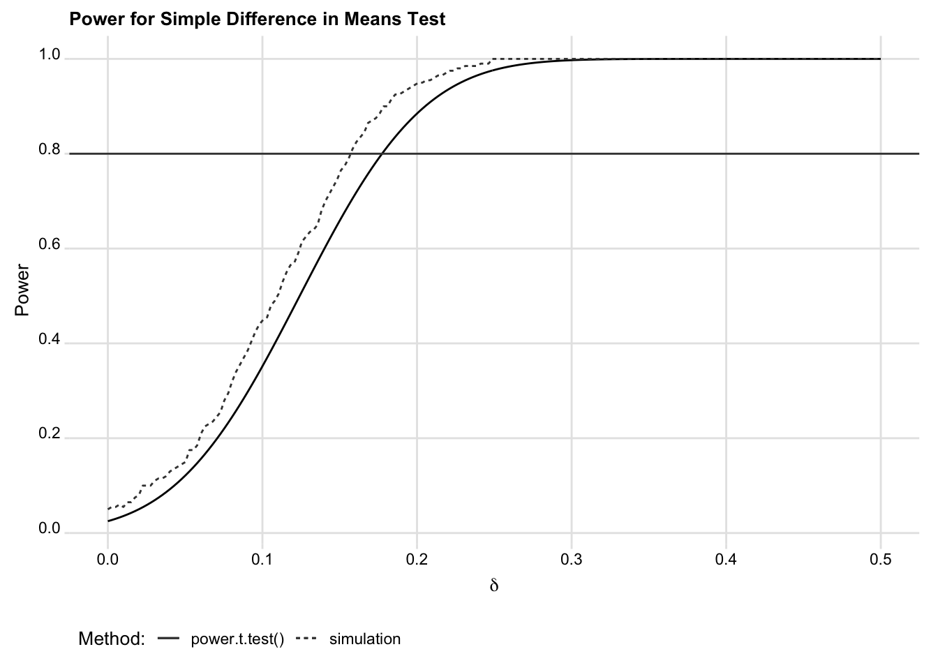
Figure 1. Off-the-shelf versus simulation power estimates
We produce these computational estimates using some helpful tools currently housed in OES’s GitHub code library and in the chunk above.
These tools are designed around a simple workflow, and remove some of the programming required to calculate power computationally.
These tools are centered around the following workflow:
- Replicate
- Estimate
- Evaluate
The first step in the workflow, Replicate, entails designing a data-generating process (which may include only an outcome variable and treatment assignment) and simulating this process multiple times to create randomly drawn datasets from a population. Each of these is a sample replicate.
The next step, Estimate, entails estimating effects for select treatments under the null hypothesis for each sample replicate. This provides a distribution of test statistics under the null hypothesis.
Finally, the last step, Evaluate, entails evaluating power to detect an effect over a range of alternative effect sizes.
This workflow is supported by three functions: replicate_design(),
estimate(), and evaluate_power(). Here’s the script used to generate the
computational estimates shown in Figure 1:
# 1. Replicate:

rep <- replicate_design(
  R = 200, # Number of sample replicates
  N = 1000, # Sample size of each replicate
  y = rnorm(N), # Normally distributed response
  x = rbinom(N, 1, 0.5) # Binary treatment indicator
)

# 2. Estimate:

est <- estimate(
  y ~ x,
  vars = "x", data = rep
)

# 3. Evaluate:

pwr_eval_sim <- evaluate_power(
  data = est,
  delta = seq(0, 0.5, len = 200)
)
The final product of this approach, the object pwr_eval_sim, reports the power
for each of the user-specified effect sizes (delta) for each of the model
terms specified by the vars command in the estimate() function. The output can
be used to plot power curves or to compute minimum detectable effects.
This approach makes computational power analysis vastly more efficient from a
programming perspective, while also providing ample room for flexibility in both
design and estimation strategy. For example, replicate_design() is a wrapper
for fabricate() in the fabricatr
package. This gives users the ability to generate multi-level or nested
data-generating processes, specify covariates, or determine whether treatment
randomization is done within blocks or by clusters. Additionally, by default,
estimates are returned using lm_robust() from the
estimatr package, but alternative
estimators can be specified. Say, for example, you have a binary response and a
set of covariates and your design calls for using logistic regression. You can
generate estimates for such a design as follows:
logit <- function(...) {
  glm(..., family = binomial)
}
est <- estimate(
  y ~ x + z1 + z2,
  data = rep, estimator = logit
)
These tools, in short, while imposing a particular workflow, provide significant latitude in terms of design and estimation. However, other tools exist as well. DeclareDesign provides useful tools, for example. And there is no shortage of simulation examples online of a variety of research designs.
8.3 When to use which approach
Of course, for a simple difference in means test, the programming required for an analytical solution is much much less involved than the computational solution. When is the latter worth the extra investment?
In cases where we’re interested in the power to detect a simple difference in
means, or a difference in proportions for binary responses, it is probably
sufficient to use power.t.test() (for means) or power.prop.test() (for
proportions).
However, OES projects often involve design features or analytic strategies that are difficult to account for using off-the-shelf tools. For example, we often include covariates in our statistical models when we analyze outcomes in order to enhance the precision of our estimates of treatment effects. If the gain in precision is small, then it might not be important to account for this in power calculations in the design phase of the project. However, if we expect a substantial gain in precision due to including covariates, then we probably want to account for this in our design. The natural way to do this is by simulation, where we can include the covariates in the “replicate” and “estimate” steps. Accounting for covariates in this way is especially useful if we can use real historical or pre-treatment data that represent the correlations we expect to see between covariates and outcomes in our later analysis of the trial data.
More complex design features or analytic strategies may make investing in the simulation approach even more worthwhile, or downright necessary. Examples include heterogeneity in treatment effects, a multi-arm or factorial design, or block randomization with differing probabilities of treatment between blocks – none of which can practically be accounted for with off-the-shelf tools. In the next section, we provide some additional examples of simulations for more complex design features or analytic strategies.
8.4 Additional examples of the simulation approach
Here we provide two examples of research designs where simulation is well worth the extra effort. Attendant R code is included in the discussion to illustrate how to use tools in the code library to streamline the approach.
8.4.1 A two-by-two design with interaction
One instance where computational power analysis may be worth the investment is in assessing power for a two-by-two factorial design with an interaction. In such a design, the goal is to assess not only the power to detect main effects (the average effect of each individual treatment), but also power to detect a non-zero interaction effect between the treatments.
Say we have a design with 1,000 observations and we would like to know the effect of two treatments on a binary outcome with a baseline of 0.25. Each treatment is assigned to \(M = 500\) individuals at random, resulting in four roughly equal sized groups of observations after randomization: (1) a control group, (2) those assigned to treatment 1 but not treatment 2, (3) those assigned to treatment 2 but not treatment 1, and (4) those assigned to both treatment 1 and 2.
We can easily calculate power to detect the main effect of each treatment, in addition to their interaction, using replication, estimation, and evaluation as follows:
two_by_two <-
  # Replicate a 2x2 design
  replicate_design(
    N = 1000,
    y = rbinom(N, 1, 0.25),
    x1 = complete_ra(N, m = N / 2) - 1 / 2, # center treatment indicators
    x2 = complete_ra(N, m = N / 2) - 1 / 2
  ) %>%
  # Estimate main and interaction effects
  estimate(
    form = y ~ x1 + x2 + x1:x2,
    vars = c("x1", "x2", "x1:x2")
  ) %>%
  # Evaluate power
  evaluate_power(
    delta = seq(0, 0.25, len = 200)
  )
Using the output reported in the object two_by_two, we can easily plot the
power curves for each of the main effects and the interaction effect, as shown
in Figure 2.
ggplot(two_by_two) +
  geom_line(
    aes(delta, power, linetype = term)
  ) +
  geom_hline(
    yintercept = 0.8,
    color = "grey25",
    alpha = 0.8
  ) +
  scale_y_continuous(
    n.breaks = 6
  ) +
  labs(
    x = expression(delta),
    y = "Power",
    title = "Power for a 2x2 Design",
    linetype = "Effect for..."
  ) +
  ggridges::theme_ridges(
    font_size = 10,
    center_axis_labels = TRUE
  ) +
  theme(
    legend.position = "bottom"
  )
Figure 2. Computational power analysis for a \(2\times 2\) design.
Of course, we could have relied on some reasonable analytical assumptions to arrive at these estimates without resorting to simulation (see a helpful discussion here), but running a simulation saves us the trouble.
8.4.2 Covariate adjustment with the Lin estimator
Another scenario where computational power analysis is worth the investment is if a design calls for covariate adjustment. This is common in OES projects, and, in several instances, the Lin (2013) saturated estimator is the analytical solution employed.
Devising an off-the-shelf method to calculate power for such a study is possible, but would likely require investing time doing background research to ensure its accuracy. Alternatively, we could simply replicate, estimate, and evaluate such a design computationally. The results will be just as accurate, without the added hassle of programming the appropriate analytical solution.
Suppose we have a sample of 1,000 observations and a continuous outcome variable. We wish to assess the effect of some policy intervention on this continuous outcome. Our design calls for randomly assigning \(M = 250\) individuals to receive the intervention, and the rest to control.
In addition to having data on the outcome and on treatment assignment, say that
we also anticipate obtaining a dataset of covariates for our 1,000 observations.
This data contains two variables that are prognostic of the outcome. We’ll call
these z1 and z2. The first is a continuous measure; the latter a binary
indicator. Our design calls for adjusting for these covariates via the Lin
estimator to improve the precision of our estimated treatment effect. We can
simulate such a design, and further justify covariate adjustment, using the
following replication, estimation, and evaluation.
We begin by replicating the data-generating process:
rep_data <-
  replicate_design(
    N = 1000,
    z1 = rnorm(N, sd = 3), # continuous covariate
    z2 = rbinom(N, 1, 0.25), # binary covariate
    cz1 = z1 - mean(z1), # make mean centered versions of the covariates
    cz2 = z2 - mean(z2),
    y = 0.8 * z1 - 1 * z2 + rnorm(N), # simulate the data-generating process
    x = complete_ra(N, m = N / 4) # randomly assign 25% of obs. to treatment
  )
We then estimate and evaluate. For comparison, power is computed both with covariate adjustment via the Lin estimator and without covariate adjustment:
# With the Lin Estimator
lin_adjust <-
  rep_data %>%
  estimate(
    form = y ~ x + z1 + z2 + x:cz1 + x:cz2,
    vars = "x"
  ) %>%
  evaluate_power(
    delta = seq(0, 0.5, len = 200)
  )

# With no Covariate Adjustment
no_adjust <-
  rep_data %>%
  estimate(
    form = y ~ x,
    vars = "x"
  ) %>%
  evaluate_power(
    delta = seq(0, 0.5, len = 200)
  )
We can now easily compare results under these alternative empirical strategies.
Figure 3 shows the power curves for each approach. As is clear, the Lin
estimator provides substantial improvements in power. With covariate adjustment,
we’re powered to detect an effect nearly 40% the size of the MDE without
controlling for z1 and z2. And it only took a few lines of code to get this
result.
bind_rows(
  lin_adjust %>% mutate(Method = "Lin"),
  no_adjust %>% mutate(Method = "No Covariates")
) %>%
  ggplot() +
  geom_line(
    aes(delta, power, linetype = Method)
  ) +
  geom_hline(
    yintercept = 0.8,
    color = "grey25",
    alpha = 0.8
  ) +
  scale_y_continuous(
    n.breaks = 6
  ) +
  labs(
    x = expression(delta),
    y = "Power",
    title = "Power with Lin Adjustment",
    linetype = "Method:"
  ) +
  ggridges::theme_ridges(
    font_size = 10,
    center_axis_labels = TRUE
  ) +
  theme(
    legend.position = "bottom"
  )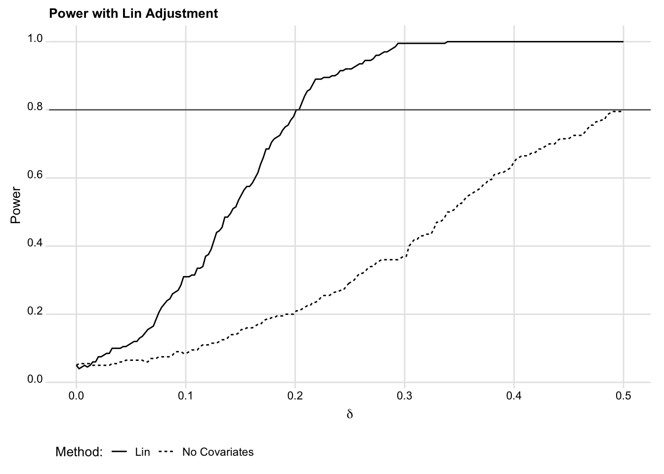
Figure 3. Simulating power with the Lin estimator.
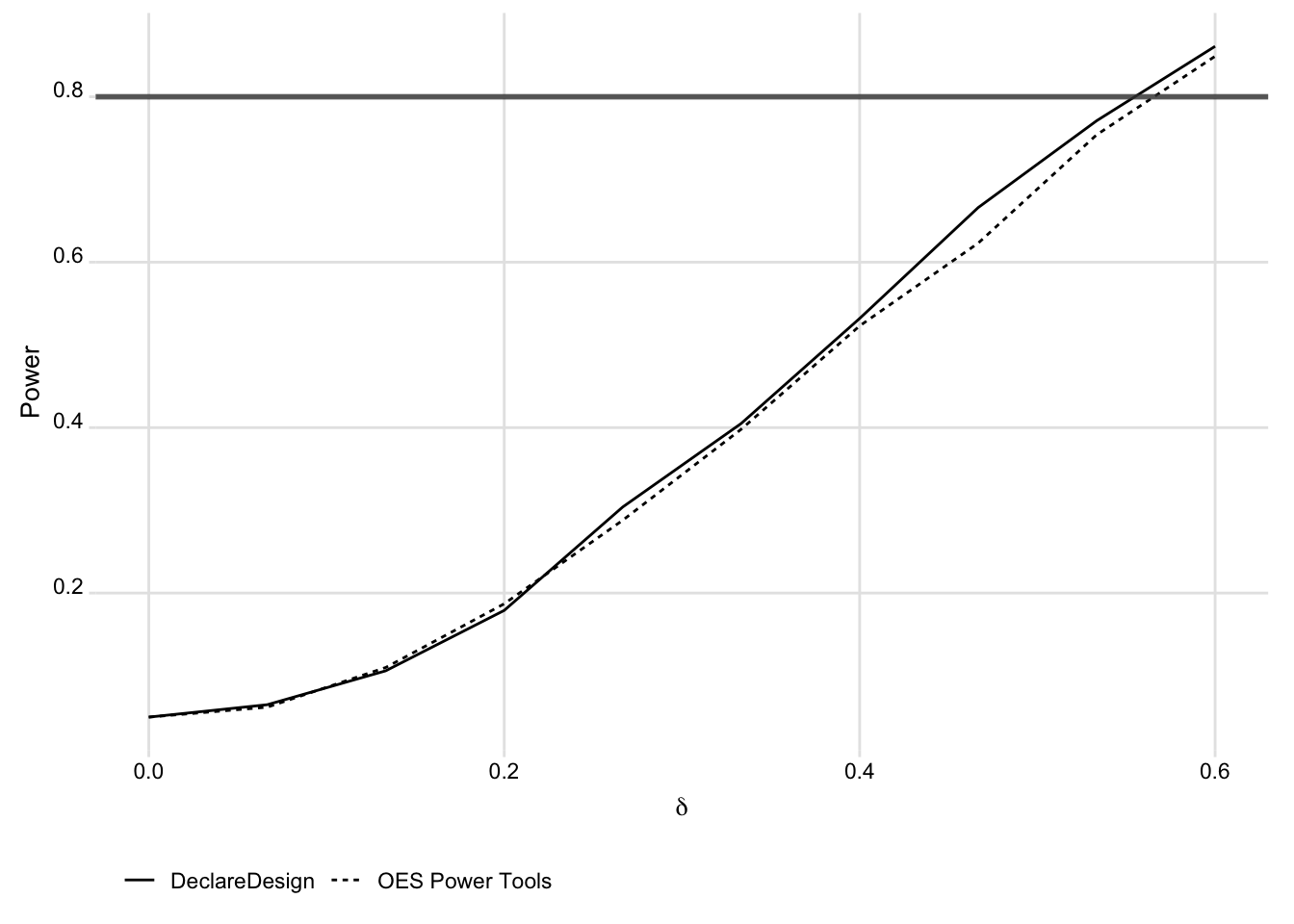
8.4.3 Incorporating DeclareDesign into OES Power Tools
We can also use DeclareDesign within the Replicate, Estimate, Evaluate framework. This involves using DeclareDesign to draw estimates, and then feeding the results into the OES evaluate_power() function. We compare the DeclareDesign approach to the OES Replicate and Estimate steps below.
First, we simulate a simple design with the OES tools:
eval <-
  replicate_design(
    R = 1000,
    N = 100,
    Y = rnorm(N),
    Z = rbinom(N, 1, 0.5)
  ) %>%
  estimate(
    form = Y ~ Z, vars = "Z"
  ) %>%
  evaluate_power(
    delta = seq(0, 0.6, len = 10)
  )
Then, we do the same with DeclareDesign, declaring a population, potential outcomes, assignments, a target quantity of interest, and an estimator:
design <- declare_population(
  N = 100,
  U = rnorm(N)
) +
  declare_potential_outcomes(
    Y ~ 0 * Z + U
  ) +
  declare_assignment(Z = complete_ra(N,
    prob = 0.5
  )) +
  declare_inquiry(ATE = mean(Y_Z_1 - Y_Z_0)) +
  declare_measurement(Y = reveal_outcomes(Y ~ Z)) +
  declare_estimator(
    Y ~ Z,
    inquiry = "ATE",
    model = lm_robust
  )
We then use draws from this design within the OES tools:
dd_eval <- replicate(
  n = 1000,
  expr = draw_estimates(design) %>%
    list()
) %>%
  bind_rows() %>%
  evaluate_power(
    delta = seq(0, 0.6, len = 10)
  )
We show the similarity between the two approaches to generating the simulated data in the figure below.
bind_rows(
  eval %>% mutate(method = "OES Power Tools"),
  dd_eval %>% mutate(method = "DeclareDesign")
) %>%
  ggplot() +
  geom_line(
    aes(delta, power, linetype = method)
  ) +
  labs(
    x = expression(delta),
    y = "Power",
    linetype = NULL
  ) +
  scale_y_continuous(
    n.breaks = 6
  ) +
  geom_hline(
    yintercept = 0.8,
    col = "grey25",
    size = 1,
    alpha = 0.8
  ) +
  ggridges::theme_ridges(
    center_axis_labels = TRUE,
    font_size = 10
  ) +
  theme(
    legend.position = "bottom"
  )